Black box Security
Measuring security via Machine Learning
Last updated: 19th August 2018
In the paper “Bayes, not Naïve: Security Bounds on Website Fingerprinting Defenses” (Cherubin, 2017) we introduced a method to quantify the security of defences to Website Fingerprinting (WF) attacks: security bounds for a WF defence can be derived, with respect to a set of state-of-the-art features an adversary uses, by computing an estimate \(\eta\) of the Bayes error on a dataset of defended network traces; we showed that an estimate based on the Nearest Neighbour classifier works well. We also proposed a security parameter, \(\varepsilon\), which measures how better than random guessing an adversary can achieve.
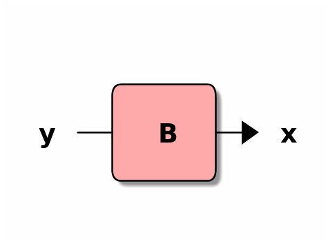
However, the method is applicable to a much more general problem: suppose to have a black-box taking some secret input \(y \in Y\) and returning some output \(x \in X\) accordingly; also, assume that the output \(x\), given some value \(y\), takes values from some (unknown) probability density function \(f_y\).
The method we introduced allows estimating the smallest error an adversary makes when trying to predict \(y\) given \(x\). Furthermore, the resulting security parameter \(\varepsilon\) conveys properties that generalise such bounds to adversaries with prior knowledge.
This page collects FAQs and future developments of this work. It does not go into depth with the specific application of the method to WF, whose details you may find in (Cherubin, 2017) and the respective talk, but it attempts to be a guide for someone looking to apply the same approach to other problems. It is also based on recent work with Catuscia Palamidessi and Kostas Chatzikokolakis, currently under submission (Cherubin et al., 2019).
I gave a talk summarising some of the contents of this page at the Turing Institute, which you may find here.
The FAQs are preceded by a short intro, which gives a high level idea of the threat model and the method, and guides the reading of the FAQs by providing links to the appropriate sections. The last question answered in the FAQs gives a Python example of how to compute the bounds for some black-box in practice.
- Prelude
- FAQs
- What is \(\eta\)?
- What is \(\varepsilon\)?
- Any assumptions on the underlying distribution?
- I don’t like asymptotic results, can I prove a rate of convergence?
- What if I (don’t) know the priors?
- What if the adversary has external knowledge?
- The NN classifier is defined for some metric: which one should I use?
- So, is NN, like, the best classifier ever?
- Other ways to estimate \(\eta\)?
- Other approaches?
- Features?
- Relabelling (e.g., Open World scenario in WF attacks)
- When should I use this method?
- Enough theory! How do I use this thing?
- Epilogue
Prelude
Threat model
We consider a finite secret space \(Y={1, 2, ..., L}\). The case of infinite and uncountable \(Y\) is currently outside the scope of this FAQ, although similar results to the ones shown here can be proven under those conditions.
We consider a black-box, \(B: Y \mapsto X\), with \(X=\mathbb{R}^d\) and \(d>0\); \(B\) is a randomised algorithm, which for some input \(y \in Y\) returns an observation \(x \in X\) according to a probability density \(f_y\). We assume that such density does not change over time (i.e., between queries to the black-box), but we make no further assumptions on its nature. “To sample” \(B\) for some secret \(y\) will mean that we sample an observation \(x\) according to \(f_y\). Secrets \(y\) are chosen according to some priors \(P(y)\); again, no assumption over the priors’ distribution is required to formulate security guarantees, and uniform priors can be used instead; if for some application priors are known, one can specify them instead of using uniform ones.
          ----------
          |////////|
          y -->|// B ///|--> x
          |////////|
          ----------
In a training phase, an adversary is given oracle access to the black-box, which he can sample \(n\) times for desired labels \(y_i \in Y\) to obtain the respective observations \(x_i \in X\). In a test phase, a secret \(y \in Y\) is chosen according to the priors, the adversary is given an observation \(x\) obtained by sampling \(B\) for secret \(y\), and he is asked to make a prediction \(\hat{y}\) for the secret. It is useful to remark that examples \((x_i, y_i)\) sampled in this way are independent, and they come from a joint distribution over \(X\times Y\) that is defined by the priors and the probability densities \(f_y\).
The adversary “wins” if \(y=\hat{y}\). In what follows, we will generally refer to the adversary’s probability of error; that is, \(P(y\neq\hat{y})\) for one run of this attack.
Computing security bound \(\eta\) and parameter \(\varepsilon\)
In the FAQs below, we will indicate that the probability of error of an adversary is lower-bounded by the Bayes error \(R^*\), which we can estimate by using ML methods; we indicate an estimate of \(R^*\) with \(\eta\). Furthermore, we derive a security parameter \(\varepsilon\), which depends on \(\eta\) and the prior probabilities, and which can be used to quantify the leakage of the black-box. Follows an intuition of the method.
To measure the smallest probability of error \(\eta\) achievable by an adversary and the respective security parameter \(\varepsilon\) of a black-box \(B\), one can proceed as follows:
- create a dataset of \(n\) examples \((x_i, y_i)\) by sampling the black-box repeatedly for various \(y_i\); secrets \(y_i\) should be chosen either: i) according to the real priors, if they are known, ii) uniformly at random;
- estimate \(\eta\) on such dataset (e.g., by using the NN bound by Cover and Hart)
- determine \(\varepsilon\)
We then call \(\varepsilon\)-secure (or \(\varepsilon\)-private) a black-box with security parameter \(\varepsilon\).
Depending on the black-box, the estimated security bound \(\eta\) may not converge quickly enough to \(R^*\) (e.g., because the observation space \(X\) is high dimensional and difficult to separate). In this case, one may need to map the original observations \(x \in X\) into a different space \(X'\) before computing \(\eta\), by using a set of transformations \(\Phi: X \mapsto X'\) called features; our application of the method to WF required doing this (Cherubin, 2017). If \(\eta\) (and, consequently, \(\varepsilon\)) are computed after extracting features \(\Phi\), we will talk about \((\varepsilon, \Phi)\)-secure (or \((\varepsilon, \Phi)\)-private) black-boxes.
FAQs
What is \(\eta\)?
The Bayes risk \(R^*\) is the smallest error that any classifier (even if computationally unbounded) can achieve on a dataset (Cherubin, 2017); in our context, it is the smallest error that any adversary may commit at separating examples coming from the distribution on \(X \times Y\). In practice, it is generally not possible to know the real Bayes risk, as this would require knowledge of the underlying probability distributions.
We call \(\eta\) an estimate of the Bayes risk \(R^*\), and thus an estimate of the smallest error that an adversary can commit.
In the original paper (Cherubin, 2017), we used an estimate \(\eta\) that is computed as a function of the Nearest Neighbour (NN) classifier’s error \(R^{NN}\) and the number of unique labels \(L = |Y|\) as follows:
\[\eta := \frac{L-1}{L} \left(1-\sqrt{1-\frac{L}{L-1}R^{NN}}\right)\]This estimate comes from a beautiful paper by Cover and Hart (“Nearest Neighbor Pattern Classification,” 1967), who show that, as the size \(n\) of the dataset on which we compute the NN error grows, the following is true:
\[\eta \leq R^*\]\(\eta\) computed this way is actually a lower bound of \(R^*\) rather than a proper estimate; this was a conservative choice due to the application. Other ways exist to estimate \(\eta\).
What is \(\varepsilon\)?
The security parameter \(\varepsilon \in [0, 1]\) indicates the advantage that an adversary has w.r.t. random guessing, and it measures the black-box’s leakage. It is defined as follows:
\[\varepsilon = \frac{\eta}{R^G}\]where \(R^G\) is the random guessing error (i.e., the error committed when random guessing according to priors). The parameter \(\varepsilon\) takes value \(1\) for a perfectly private defence (i.e., one that forces an adversary into random guessing), \(0\) where there may exist an attack achieving \(0\) error.
\(\varepsilon\) is also related to well-known security and privacy parameters, from which it inherits interesting properties.
-
\(\varepsilon\) corresponds, in the binary case (\(L=2\)) with uniform priors (hence, \(R^G = 0.5\)), to \(1 - Adv\), where \(Adv\) is the advantage as it is commonly used in Cryptography. In cryptographic proofs, \(Adv\) is usually derived analytically from a security game, and then shown to be negligibly small. In our case, it is the result of a measurement (\(\eta\)).
-
\(\varepsilon\) is also related to the Multiplicative Leakage \(\mathcal{ML}\), introduced in Quantitative Information Flow (QIF), which measures the leakage of a channel (Braun et al., 2009); differently from \(\varepsilon\), \(\mathcal{ML}\) is defined in terms of an adversary’s success probability rather than his error: \(\mathcal{ML} = \frac{1 - \eta}{1 - R^G}\). However, \(\mathcal{ML}\) has an interesting property which \(\varepsilon\) does not satisfy in general: \(\mathcal{ML}\) computed for uniform priors is an upper bound on the multiplicative leakage computed for any other set of priors (note that \(\mathcal{ML}\) is larger the more the system leaks). This is called the “Bayes capacity theorem”.
Any assumptions on the underlying distribution?
Nope. So long as examples \((x_i, y_i)\) are sampled i.i.d. (which is the case in the game we defined), \(R^*\) is a lower bound for any distribution on \(X \times Y\), and the guarantees we derive on \(\eta\) are valid.
Specific estimates \(\eta\) may make very weak assumptions on the distribution or the observation space. For example, the NN estimate requires continuity of densities \(f_y\) and a separable metric space; both are generally satisfied in real-world applications.
I don’t like asymptotic results, can I prove a rate of convergence?
Unfortunately, no.
Impossibility result. Antos et al. (“Lower Bounds for Bayes Error Estimation,” 1999) showed that, for any estimate \(\eta\) of the Bayes risk, it is possible to find probability distributions for which such estimate converges arbitrarily slowly to \(R^*\) as \(n\) increases.
Hence, estimating the security of a black-box via measurements will never give convergence guarantees. This means we can never be completely sure of the performances of a Bayes risk estimate \(\eta\): under no further assumptions on the distribution, no such estimate can be proven to converge at a certain rate. In the paper, we used the following heuristics to determine convergence:
- visually inspect that the trend of \(\eta\) becomes stable as \(n\) increases
- verify that \(\eta\) is smaller than the error of other classifiers.
Clearly, if more information was available on the actual priors/distribution, this could be used for estimating \(R^*\) more precisely and to obtain convergence rate guarantees.
What if I (don’t) know the priors?
In general, you may want to use a leakage measure for which the “Bayes capacity theorem” (Braun et al., 2009) holds, which means the leakage measure is minimised (or maximised, depending on the formulation) when computed for uniform priors.
Multiplicative leakage, \(\mathcal{ML} = \frac{1 - η}{1 - R^G}\), is an example of this: if one computes \(\mathcal{ML}\) for uniform priors, then they achieve an upper bound on the black-box’s leakage.
This means that, even if we don’t know the true priors over \(Y\), we can use uniform priors to obtain strong security guarantees. However, when we actually know the real priors, we can use them instead to get a more tight security estimate.
The same result does not hold for \(\varepsilon\) in the general case \(L>=2\), although \(\varepsilon\) does give these guarantees in a restricted case. This is ongoing research, and more will follow.
What if the adversary has external knowledge?
In some attacks, the adversary can exploit external knowledge. For instance, in some definition of WF attacks, an adversary may link multiple test observations by assuming they correspond to web pages of the same website.
The security parameter \(\varepsilon\) is an indication of the leakage of the black-box itself. While it is clearly impossible to determine security against any adversary with external knowledge (trivially, one such adversary is an adversary who already knows the secret), one can use black-box measurements as a building block to prove the security of more complex systems.
The NN classifier is defined for some metric: which one should I use?
The lower bound guarantee of the estimate \(\eta\) based on the NN classifier holds for any metric \(d\) on \(X\), with the only constraint that the metric space \((d, X)\) is separable (Cherubin et al., 2019).
In the original paper (Cherubin, 2017) we experimented with a few metrics, and opted for Euclidean.
So, is NN, like, the best classifier ever?
No.
1) Note that we use a transformation of the actual NN classifier’s error as a security bound. \(R^{NN}\) is not guaranteed to converge to \(R^*\).
2) BUT, for example, the error of the k-NN classifier, with \(k\) increasing with \(n\) according to some requirements (Appendix in (Cherubin, 2017)), does converge asymptotically to \(R^*\). Classifiers satisfying such property are called universally consistent. However, no classifier can guarantee on its performance in the finite sample under no assumptions over the distribution (No Free Lunch theorem), and thus there is no such thing as the “best classifier ever”.
Other ways to estimate \(\eta\)?
Plenty. The error of any universally consistent classifier will converge to \(R^*\) asymptotically in the number of training examples \(n\).
Examples of universally consistent classifiers:
- k-NN classier with the following properties. As \(n \rightarrow \infty\): \(k \rightarrow \infty\) and \(k / n \rightarrow 0\)
- SVM with appropriate choice of kernel.
Other approaches?
Measuring the security of a black-box \(B\) means telling something about how hard it is to separate the probability distributions \(B\) defines on \(X \times Y\).
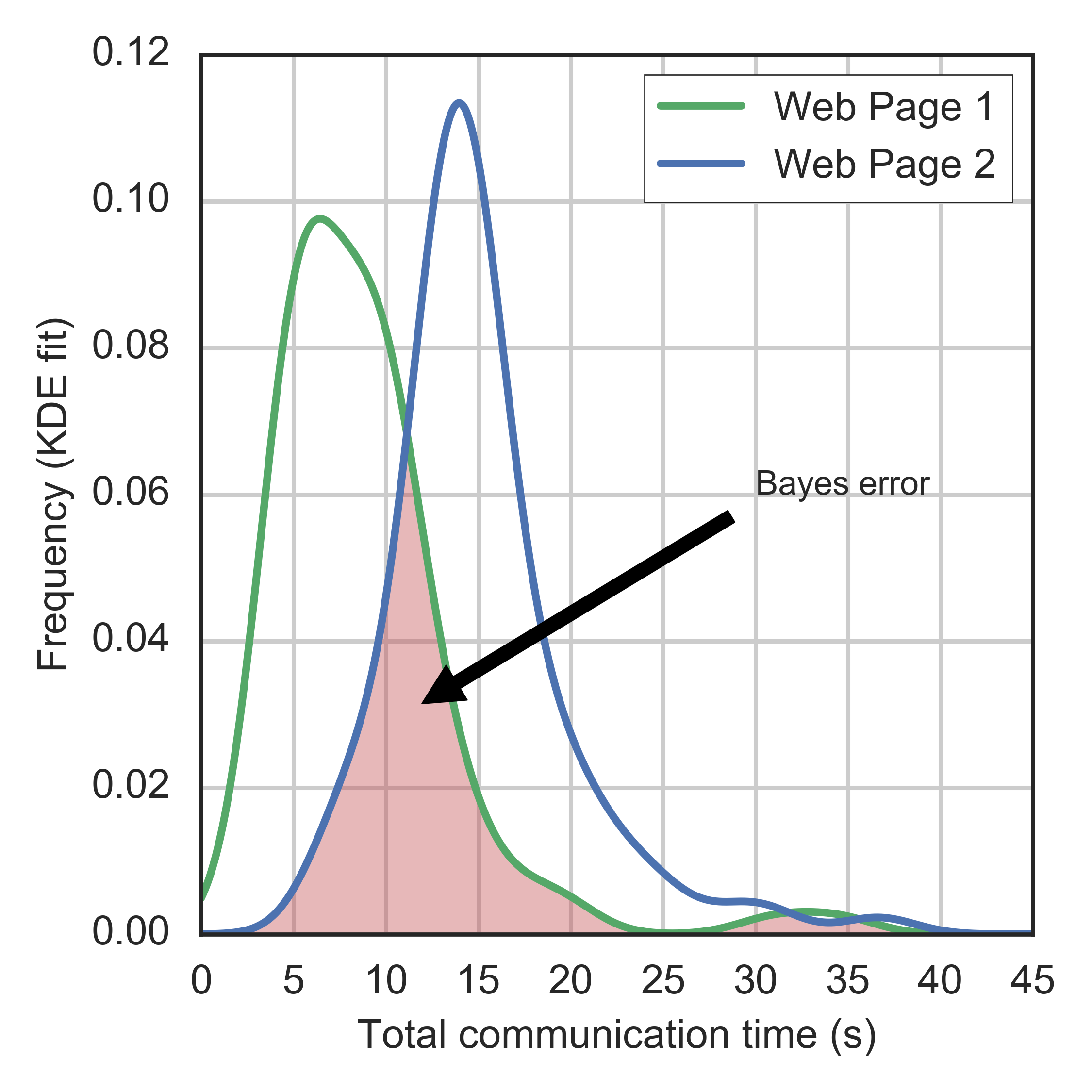
Clearly, an estimate of the Bayes risk is not the only strategy. For instance, one may estimate the information leakage of the black-box by using a statistical test on the distributions (e.g., Kolmogorov-Smirnov test), or by estimating the distributions directly (e.g., using KDE).
The advantage of our approach (i.e., using a universally consistent classifier to estimate \(R^*\)) is that it outputs a probability of error, whose meaning we argue is more intuitive than a statistic on the distributions’ distance.
Also, note that by using the NN (or k-NN) classifier, we are essentially approximating the underlying probability distributions (k-NN methods are indeed based on the intuition that the posterior density at some point can be approximated by the posterior of its neighbours).
Features?
Because a Bayes risk estimate \(\eta\) may not converge in practice, one may need to map observations \(x_i \in X\) into some new space \(X'\) called the feature space to improve the estimate’s convergence.
In fact, while asymptotically the estimate in the original space \(X\) will never be worse than the estimate in the feature space (see 5.6 in (Cherubin, 2017)), this may be the case in finite sample conditions.
If this is the case, one will need to select good features, and the achieved \((\varepsilon, \Phi)\)-security (where \(\Phi\) indicates the mapping from \(X\) into \(X'\)) will only hold until a better mapping \(\Phi''\) is found. In the context of WF (Cherubin, 2017), we worked in the feature space, and argued that finding better features is becoming harder.
Relabelling (e.g., Open World scenario in WF attacks)
Remapping the secrets (i.e., “relabelling”) may be useful to adapt a black-box to different scenarios.
Consider a setting where there are \(L=100\) secrets, and then consider the following distinct attack scenarios:
- the adversary has to guess the exact secret
- the adversary needs to output \(0\) if he believes the secret is below \(50\), and \(1\) otherwise.
To model the first case, we will simply consider a black-box \(B: \{1, 2, ..., 100\} \mapsto X\). To model the latter, we can remap the secrets into \(\{0, 1\}\), so that the secret is \(0\) if the original secret is below \(50\), \(1\) otherwise; then we define a black-box \(B: \{0, 1\} \mapsto X\), and measure its security as usual.
The idea of relabelling allows defining various scenarios for attacks. In the context of WF, we used this to define the Open World scenario (where the adversary needs to predict whether a web page is among a set of monitored web pages or not), as opposed to the Closed World scenario (where the adversary needs to predict the exact web page). Variations of the Open World scenario can be defined similarly.
Remark on evaluating WF in Open World scenario Even though we can determine \((\varepsilon, \Phi)\)-privacy in an Open World scenario, we recommend against: such metric should be computed under optimal conditions for an adversary (a Closed World scenario) (Cherubin, 2017).
When should I use this method?
There are two strategies for quantifying the security of a black-box:
- if the internals of the black-box are known (e.g., its internal probability distribution), one can try to derive a concrete proof of its security; this is to be preferred whenever possible (see below);
- if concrete proofs are not viable (e.g., think of side channel attacks), one can measure its security by using a black-box estimate of the Bayes risk.
Clearly, if one can easily model the system’s internals, the former is encouraged; indeed, it is not possible to prove convergence for the latter under our relaxed assumptions. However, there are many real-world problems for which black-box approaches would seem to be the only candidate; and indeed, the convergence of our methods is achieved for several of them.
Note that both strategies have been widely explored in Cryptography and QIF. To the best of our knowledge, the extension to infinite spaces \(X\) was not tackled until now, and we showed it is achieved by any universally consistent learning algorithm.
Enough theory! How do I use this thing?
Clone the GitHub repo and
cd into code/.
Sample your black-box many times to obtain a dataset of observations \(x_i\) and labels \(y_i\). Then:
    import numpy as np
    from scipy.spatial.distance import pdist, squareform

    from evaluate.bounds import nn_bound_cv

    # Say you have the following dataset of observations (X) and respective
    # labels (Y), sampled from a black-box.
    X = np.array([[1, 2], [2, 1], [1, 1], ...])
    Y = np.array([0, 0, 1, ...])

    # Compute pairwise distances for some metric. This step just makes it
    # more efficient to run Nearest Neighbours afterwards.
    D = squareform(pdist(X, metric='euclidean'))

    # Compute the bound $$\eta$$ using 5-folds CV, and averaging the results.
    bounds = nn_bound_cv(D, Y, n_folds=5)
    eta = np.mean(bounds)

    # Compute the security parameter $$\varepsilon$$, assuming uniform priors.
    # See below if priors are not uniform.
    L = float(len(np.unique(Y)))            # Number of labels
    Rg = (L - 1)/L                          # Random guessing error
    epsilon = eta / Rg                      # Security parameter
The estimate will be based on the NN bound. We plan to support other methods in the future.
We suggest plotting the value of eta as you let increase the size of the
dataset. This will give you an indication regarding the convergence
of the estimate (see (Cherubin, 2017)).
Should you have non uniform priors, set Rg = 1 - max(P(y)).
However, consider
what discussed about priors.
Epilogue
Changes
As there will probably be mistakes/imprecisions, I will welcome feedbacks and corrections (see the homepage for my contact details), which I will report here.
- 19/08/2018 The ““Bayes capacity theorem”” (i.e., a leakage measure is minimised/maximised by uniform priors) does not hold in general for \(\varepsilon\), although it does hold for \(\mathcal{ML}\).
References
-
Quantitative notions of leakage for one-try attacks Electronic Notes in Theoretical Computer Science 2009
-
Lower bounds for Bayes error estimation IEEE Transactions on Pattern Analysis and Machine Intelligence 1999